Weather Calculations

Atmospheric Model Grids

A grid of atmospheric temperature and opacity were calculated using *am* models for the Atacama Plateau (specifically using the configuration files for the Atacama Cosmology Telescope). The grids are created at water profile percentiles of 5%, 25%, 50%, 75% and 95% (where the percentiles indicate the percentage of time when the conditions are at least as dry as in the corresponding grid - see below for a conversion to precipitable water vapour). These grids contain the Rayleigh-Jeans brightness temperature of the sky, \(T_\mathrm{sky}(z=0)\) and the sky opacity, \(\tau_0\), where these are both calculated at zenith. These are then interpolated to the observing frequency and percentile water column requested in the sensitivity calculator. In order to adjust these to the chosen elevation, the code calculates the atmospheric temperature, \(T_\mathrm{atm}\), and transmittance \(\mathfrak{t}\) as a function of the zenith angle (90°-elevation)

\[T_\mathrm{atm} = \frac{T_\mathrm{sky}(z=0)}{1-e^{-\tau_0}}\]

and the transmittance as a function of the zenith angle (90°-elevation)

\[\mathfrak{t} = e^{-\tau_0\sec{z}}\]

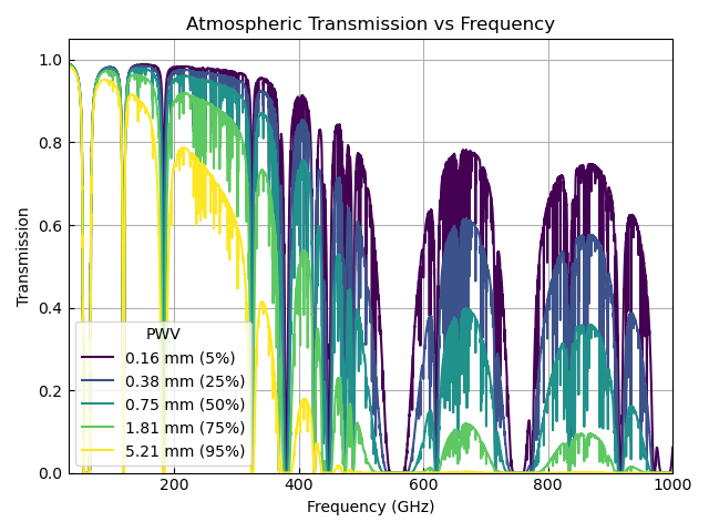
The transmittance for the different weather conditions as a function of frequency is shown in the following figure

The sky temperature at the chosen elevation is then calculated from these terms. At this stage, the contribution from the temperature of the Cosmic Microwave Background, \(T_\mathrm{cmb}\), is also added, noting that this needs to be converted to a Rayleigh-Jeans brightness temperature for consistency.

\[T_{sky} = (1-\mathfrak{t})\times T_{atm} + O(\nu, T_\mathrm{cmb})\]

Here, \(O(\nu, T)\) converts a physical temperature to a Rayleigh-Jeans brightness temperature

\[O(\nu, T) = T\frac{h\nu/kT}{\exp(h\nu/kT)-1}\]

where \(\nu\) is the observing frequency, \(h\) is the Planck constant and \(k\) is the Boltzmann constant.

Percentile Water Profile to Precipitable Water Vapour

The input required for the calculator is the percentile water profile of the atmosphere, which takes a value between 5 and 95%, with 5% being very dry conditions that only occur 5% of the time and 95% being very wet conditions.

These percentiles map to the precipitable water vapour (PWV) based on the pressures and volume mixing ratios in the am configuration files as shown in the following table.

Percentile water profile to PWV

Water Profile - (%)	PWV - (mm)
5.00	0.16
25.00	0.38
50.00	0.75
75.00	1.81
95.00	5.21

Atmospheric windows

As can be seen from the transmission plot above, there are regions of high transmission that provide the atmospheric windows. Di Mascolo et al. 2025 investigated the maximum bandwidth for each window, making use of the finetune parameter for broadband sensitivity, which we show in the table below as a guide for the maximum bandwidth that should be used when setting up continuum observations. Note that this only takes into account the impact due to the atmosphere. In reality, continuum cameras will often have a lower bandwidth than this due to aspects of the instruments themselves, such as the design of the filters. For instance, MUSCAT has a bandwidth of 45 GHz with a central frequency of 277.5 GHz. See the instrument overview and individual instrument pages for further details on the ranges of bandwidths they can cover.

Central frequency and maximum bandwidth for the atmospheric windows

Central frequency - (GHz)	Bandwidth - (GHz)
42.0	24
91.5	51
151.0	62
217.5	69
288.5	73
350.0	50
403.0	38
654.0	118
845.5	119